The Lorenz system is a system of three ordinary differential equations which exhibits chaotic solutions for certain initial conditions and parameter values. The system is based on a simple model of convection, studied by the mateorologist Edward Lorenz. The system has two fixed points other than the origin: for some values the solution will spiral towards one of those fixed points, for others the solution becomes chaotic, orbiting the first one fixed point, then another.
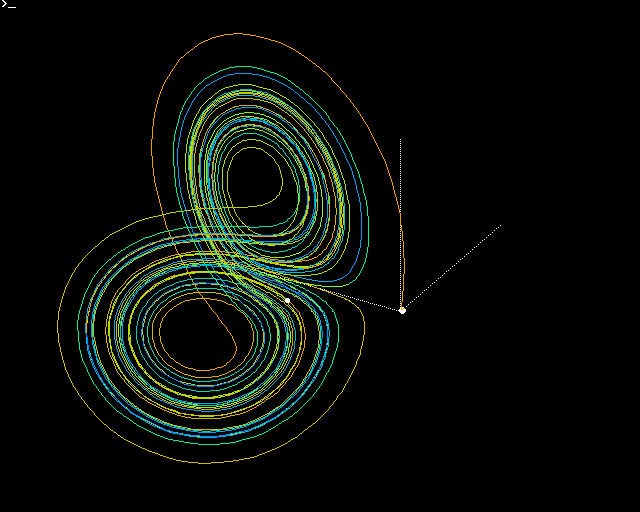
The construction is based on the following differential equations:
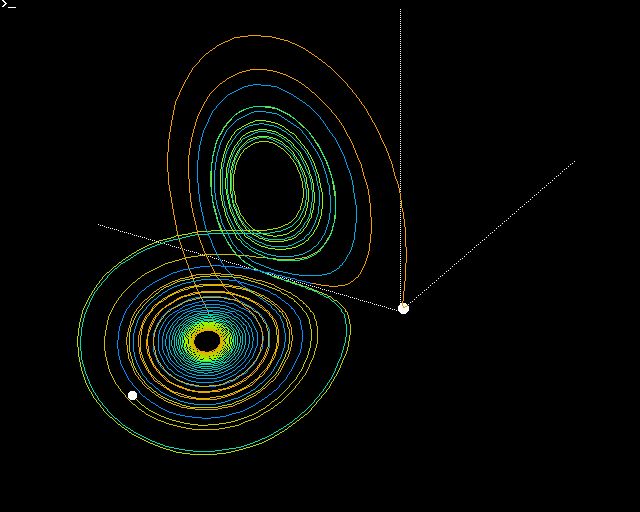
Starting with the initial value (1, 0, 0) and solving the system numerically, proceed to plot the solution obtained for each time step as a point in three-dimensional space. In the above image I have adopted the convention of taking the z axis as pointing into the display. The image is then rotated around the x and y axis to better show the resulting curve. The points are coloured, from orange through green to blue, to show the time value. The sequence of colours repeats as necessary. The time variable t ranges between 0 and 32, and the axes, shown as dotted white lines, are each 50 units long. The usual values for the constant parameters are: rho=28, sigma=10 and beta=8/3.
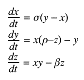
A chaotic system is essentially a deterministic system which shows great sensitivity to initial conditions. This is true of the Lorenz system, and by starting from (1, 0, 1) instead, the following curve is obtained. Although its overall shape is similar, the exact trajectory is completely different, as will be seen by comparing the start and end points shown by small white circles:
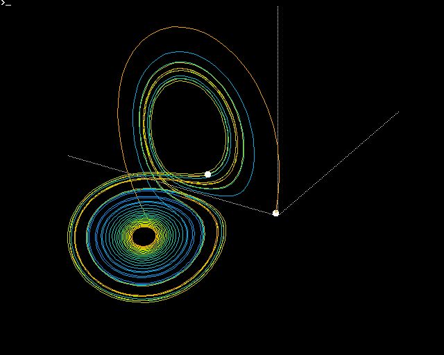
More variation can be obtained by using different values of the constant parameters. For example, taking rho=50, sigma=10 and beta=4, the following curve is obtained. It has been necessary to reduce the scale in order to fit the display, and the time variable only runs as far as 24:
The following program in the Julia programming language will calculate the trajectory of the Lorenz system, although there is no graphics as yet. The function main repeatedly calls midpoint to advance the solution of the equations by one time step, using the second order midpoint method. The function lorenz evaluates the derivatives at the specified point. Although the time variable is not needed to evaluate the Lorenz system, it is passed into the two functions to emphasise that it would be necessary in the more general case.
# Constants for the Lorenz system
const rho::Float64=28.0
const sigma::Float64=10.0
const beta::Float64=8.0/3.0

# Time step
const h::Float64=1.0/128.0

# Rotation of coordinate system in radians
const xrot::Float64=30.0*pi/180.0
const yrot::Float64=60.0*pi/180.0
const scale=10

function lorenz(x::Float64, Y::Array{Float64})
    [ sigma*(Y[2]-Y[1]),
      Y[1]*(rho-Y[3])-Y[2],
      Y[1]*Y[2]-beta*Y[3] ]
end

function midpoint(x::Float64, Y::Array{Float64}, derivs)
    DY=derivs(x, Y)
    K=Y+(0.5*h)*DY
    DY=derivs(x+0.5*h, K)
    Y=Y+h*DY
end

function transform(Y::Array{Float64})
    zprime=Y[1]*sin(yrot)+Y[3]*cos(yrot)
    xprime=Y[1]*cos(yrot)-Y[3]*sin(yrot)
    yprime=Y[2]*cos(xrot)+zprime*sin(xrot)
    (round(scale*xprime), round(scale*yprime))
end

function main()
    # Initial conditions for ODEs
    Y::Array{Float64}=[1.0, 0.0, 0.0]
    t::Float64=0.0
    while t<=32
	Y=midpoint(t, Y, lorenz)
	t+=h
    end
end

main()